
Fix SUMIF/COUNTIF missing a number in Google Sheets (CHAR(160))
Both rows look like sku 101 with qty 10, yet COUNTIF returns 1 and SUMIF returns 10. The formulas ran. They only matched one row. There is no red error triangle.
Recreate it on a blank sheet
Section titled “Recreate it on a blank sheet”- Open a blank spreadsheet. Leave the tab named
Sheet1. In A1 typesku, B1qty. - In A2 enter
="101"&CHAR(160). The cell looks like 101 and sits left-aligned. In A3 type101as a number. That 101 is right-aligned. B210. B310. Both quantities are numbers. - In C1 type
len, D1trim_len, E1countif, F1sumif. In C2 enter=LEN(A2). The cell shows 4. In D2 enter=LEN(TRIM(A2)). That cell is still 4. In E2 enter=COUNTIF(A2:A3,101). The cell shows 1. In F2 enter=SUMIF(A2:A3,101,B2:B3). The cell shows 10. None of those four cells has a red error triangle.
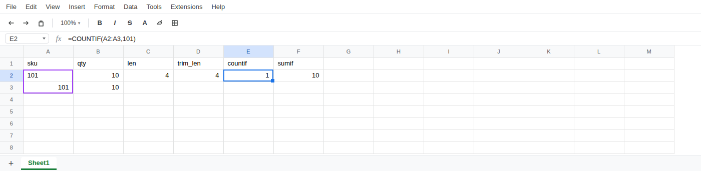
TRIMdid not strip the extra character. In J2 enter=VALUE(TRIM(A2)). That cell is#VALUE!. Do not use this as the cleanup.
What is actually wrong
Section titled “What is actually wrong”- A2 is the digits 101 plus
CHAR(160), a non-breaking space, often left over from a web paste. It looks like 101.LENis 4. TRIMremoves ordinary spaces (CHAR(32)). It does not removeCHAR(160), soLEN(TRIM(A2))stays 4.COUNTIFandSUMIFlooking for the number 101 match only A3. A2 is a different value. Qty is not missing.- This is not
'101stored as text. Sheets coerces that apostrophe-text inCOUNTIF/SUMIF. A leading apostrophe would not reproduce this miss.
Leave E2 and F2 as the broken formulas so the miss stays on the sheet.
Do not stop at VALUE(TRIM(...)). That still hits the non-breaking space and returns #VALUE!.
Clean the sku. In G1 type sku_clean. In G2 enter =VALUE(TRIM(SUBSTITUTE(A2,CHAR(160),""))) and fill down through G3. Both rows become the number 101. A3 was already a number; it stays 101.
Then count and sum the cleaned column. In H1 type countif_ok, I1 sumif_ok. In H2 enter =COUNTIF(G2:G3,101). The cell shows 2. In I2 enter =SUMIF(G2:G3,101,B2:B3). The cell shows 20.
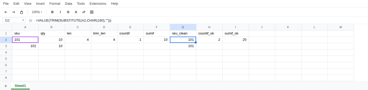
SUBSTITUTE is what removes CHAR(160). TRIM alone does not.