Look left of the key in Google Sheets (INDEX/MATCH or XLOOKUP)

You can see sku 101 on the sheet and VLOOKUP still returns #N/A. The key is a real number. It is not missing. The formula is searching the name column.

Recreate it on a blank sheet

1. Open a blank spreadsheet. Leave the tab named Sheet1. In A1 type name, B1 sku, C1 price.
2. In A2 type Widget. B2 101 as a number. C2 9.5. E1 lookup. E2 101 as a number. F1 vlookup.
3. In F2 enter =VLOOKUP(E2,A2:C2,1,FALSE). The cell shows #N/A. The tooltip is Did not find value ‘101’ in VLOOKUP evaluation.

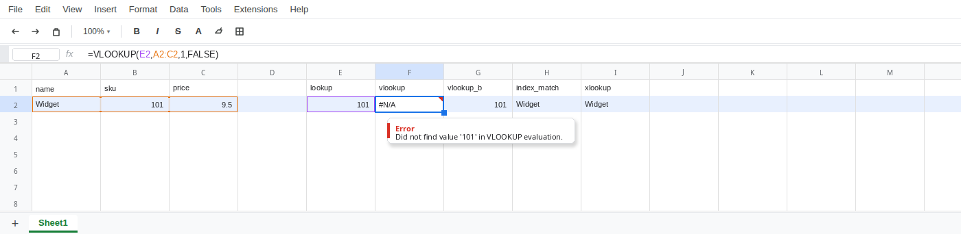
4. That is not a missing key. Start the range at sku instead. G1 vlookup_b. In G2 enter =VLOOKUP(E2,B2:C2,1,FALSE). The cell shows 101. VLOOKUP can return the search column, or columns to its right. It cannot return name.

What is actually wrong

• VLOOKUP always searches the first column of the range you give it. Range A2:C2 means it looks for 101 in A. A is Widget, not 101.
• Index 1 would return the name if it had found 101 in A. It never does.
• This is not a missing key, not a number stored as text, and not a trailing space. 101 is a number in B2 and in E2.

Fix

Leave F2 as the broken VLOOKUP. Do not move sku into column A. Leave the table as name | sku | price.

• H1 index_match. In H2 enter =INDEX(A2,MATCH(E2,B2,0)). The cell shows Widget.
• I1 xlookup. In I2 enter =XLOOKUP(E2,B2,A2). The cell shows Widget.

Both look up 101 in the sku column and return the name to the left.

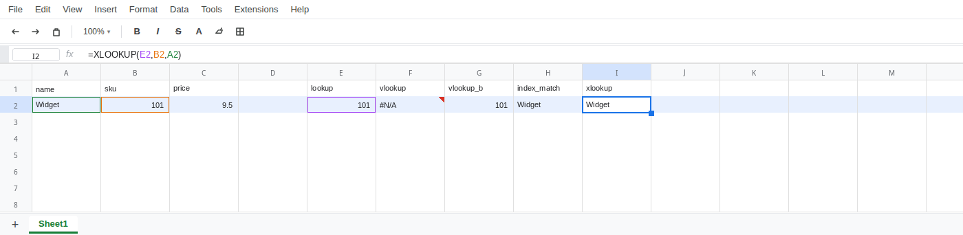
If you need a column to the left of the key, do not rearrange the table to make VLOOKUP work. Use INDEX/MATCH or XLOOKUP.