QUERY + IMPORTRANGE NO_COLUMN in Google Sheets (use Col1, not A)

QUERY around IMPORTRANGE can still show #N/A when the import already works. select A is the usual column letter. On this array it is the wrong name.

Recreate it on a blank sheet

Source sheet: A1 sku, B1 name, A2 101, B2 Widget. Leave the tab named Sheet1. On the target spreadsheet, assume IMPORTRANGE from that source already works. Paste your source id where the formulas say SOURCE_ID.
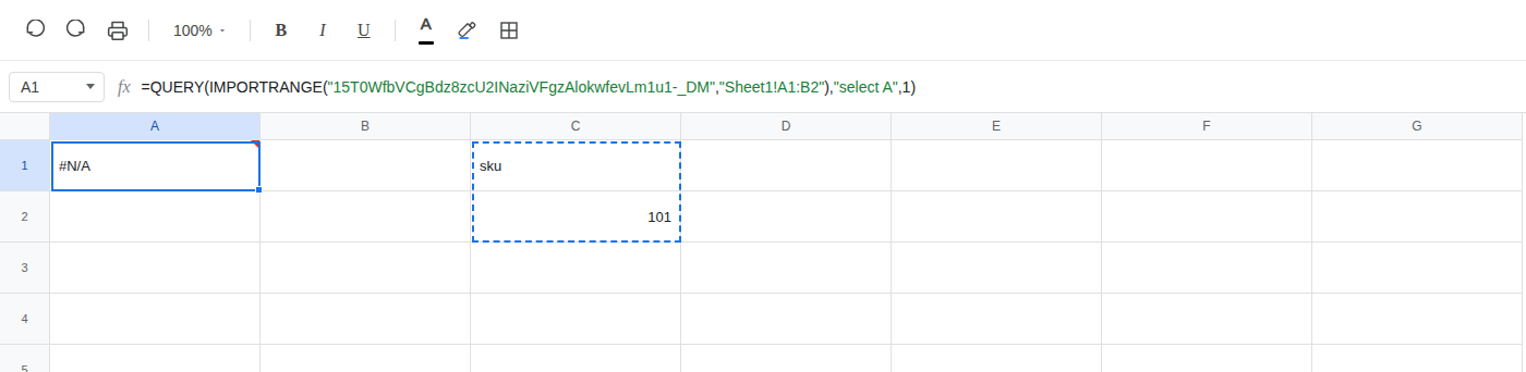
In the target, A1 enter =QUERY(IMPORTRANGE("SOURCE_ID","Sheet1!A1:B2"),"select A",1). The cell shows #N/A.

A1 selected. Formula bar shows =QUERY(IMPORTRANGE(“SOURCE_ID”,“Sheet1!A1”),“select A”,1). A1 is #N/A. C1 is sku and C2 is 101.

What is actually wrong

QUERY is reading an IMPORTRANGE array, not a sheet range. Arrays do not have column letters A and B.
select A is the syntax you use on a tab. Here it does not name a column, so the cell is #N/A. That is column syntax, not a missing lookup key.
This error is commonly reported with parse / NO_COLUMN wording. The screenshot shows #N/A in A1; it does not show hover text.

Check: =ERROR.TYPE(A1) is 7. That code is #N/A.

Fix

Change select A to select Col1. QUERY numbers IMPORTRANGE columns Col1, Col2, … from the left of the imported array.

Leave A1 as the broken formula. In C1 enter =QUERY(IMPORTRANGE("SOURCE_ID","Sheet1!A1:B2"),"select Col1",1). The formula spills sku into C1 and 101 into C2.

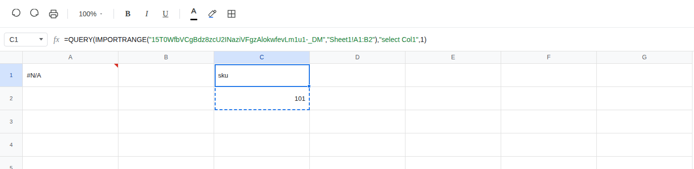
C1 selected. Formula bar shows =QUERY(IMPORTRANGE(“SOURCE_ID”,“Sheet1!A1”),“select Col1”,1). C1 is sku and C2 is 101. A1 is still #N/A.

select B becomes select Col2. Leave the rest of the QUERY as it is.