
Fix QUERY #VALUE! in Google Sheets (dates mixed with text)
Some cells in column A look like dates and QUERY still returns #VALUE!. The formula is not reading the dates you can see. It is reading the whole column’s type.
Recreate it on a blank sheet
Section titled “Recreate it on a blank sheet”- Open a blank spreadsheet. Leave the tab named
Sheet1. In A1 typedate, B1item. - In A2 type
2024/1/15so Sheets stores a real date. B2Widget. A3TBDas plain text. B3Skip. A42/1/2024as a real date. B4Gadget. A5unknown. B5Thing. A6pending. B6Doohickey. - In D1 enter exactly
=QUERY(A1:B6,"select year(A), B",1). The cell shows#VALUE!. The tooltip is Unable to parse query string for Function QUERY parameter 2: Can’t perform the function year on a column that is not a Date or a DateTime column.
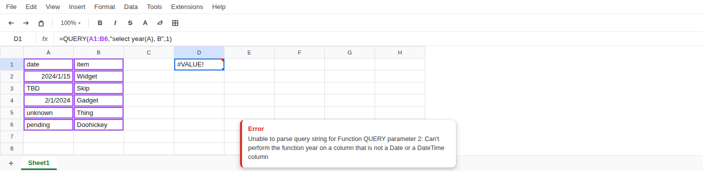
where A > date '2024-01-01' is not this recreate. On a short table that filter can succeed and hide the mixed-type problem. The recreate is year(A) on the mixed A column.
What is actually wrong
Section titled “What is actually wrong”QUERYinspects a whole column’s type. Column A mixes real dates with text (TBD,unknown,pending). That mix is not a Date or DateTime column.year(A)only runs on a Date or DateTime column. Mixed type is why the query string fails to parse.- This is not a locale / comma-vs-semicolon parse error. This is not
IMPORTRANGEselect AvsCol1.
Do not QUERY the mixed column.
Leave D1 as the broken formula so #VALUE! stays on the sheet.
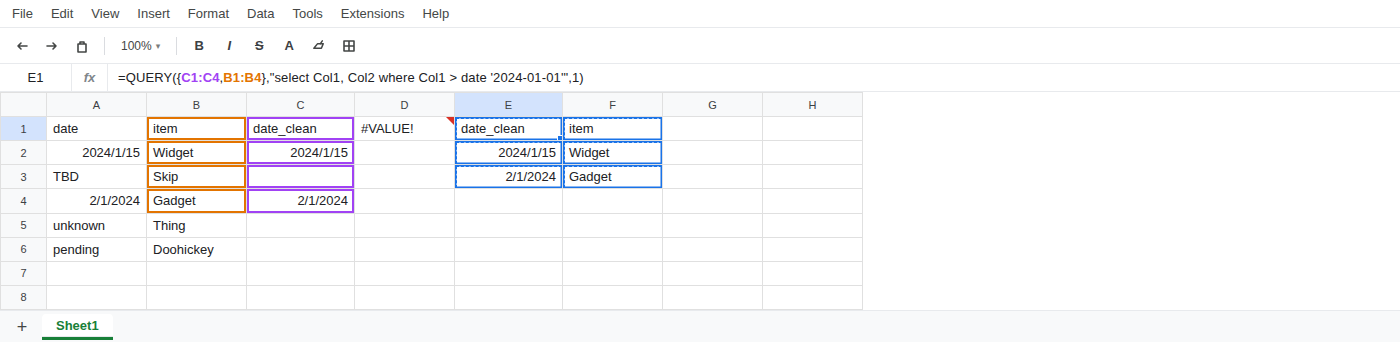
Helper column: C1 date_clean. In C2 enter =IF(ISNUMBER(A2),A2,"") and fill down through C6. Text cells become blank. Real dates remain.
Then in E1 enter =QUERY({C1:C4,B1:B4},"select Col1, Col2 where Col1 > date '2024-01-01'",1). The formula spills headers plus the two date rows: Widget and Gadget.
Do not wrap this in IMPORTRANGE. Do not change File > Settings locale. Do not try to make the mixed column one QUERY without the helper.
If year fails on a column that looks like dates, look for leftover text in that column first.